We want to study the problem of voice verification. The typical setup is constituted by brief speech segments of different individuals. These individuals have voices that sound alike. This is common in subjects like twins. The system will learn the similarity metric between subjects that are in same class for a subsequent verification step. In this scenario the number of categories is very large and not known during training, and the number of training samples for a single category is very small. The learning process minimizes a discriminative loss function that drives the similarity metric to be small for pairs of features from similar subjects, and large for pairs from different persons. The proposed architecture is a Siamese network @Bromley93. A general Siamese framework for visual recognition comprises two identical networks and one cost module. The input to the system is a pair of images and a label. The images are passed through the sub-networks, yielding two outputs which are passed to the cost module which produces the scalar energy. In speech recognition we have a different type of signal. Usually the audio signal is 1-D, instead of 2-D as for the images. In this project we are going to use two representation of the audio signal: spectrogram, and MFCC.
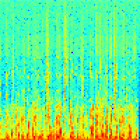
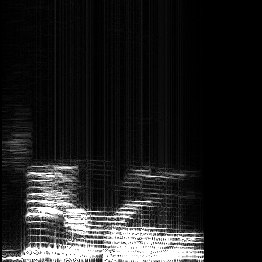
A spectrogram is a very detailed, accurate image of your audio, displayed in either 2D or 3D. Audio is shown on a graph according to time and frequency, with brightness or height indicating amplitude. Whereas a waveform shows how your signal’s amplitude changes over time, the spectrogram shows this change for every frequency component in the signal.
The mel-frequency cepstrum MFC is a representation of the short-term power spectrum of a sound, based on a linear cosine transform of a log power spectrum on a nonlinear mel scale of frequency Mel-frequency cepstral coefficients MFCCs are coefficients that collectively make up an MFC. They are derived from a type of cepstral representation of the audio clip, a nonlinear “spectrum-of-a-spectrum”. The difference between the cepstrum and the mel-frequency cepstrum is that in the MFC, the frequency bands are equally spaced on the mel scale, which approximates the human auditory system’s response more closely than the linearly-spaced frequency bands used in the normal cepstrum. This frequency warping can allow for better representation of sound, for example, in audio compression.
The difference of these two representation is the dimensionality. A spectrogram is essentially an image, thus we can use the the well known convolutional neural network used for computer vision applications. MFCC constitute a 1-D vector that need to be analyzed by a neural network with a slightly different architecture.
One of the reasons training networks is difficult is that the errors computed in backpropagation are multiplied by each other once per timestep. If the errors are small, the error quickly dies out, becoming very small; if the errors are large, they quickly become very large due to repeated multiplication. An alternative architecture built with Long Short-Term Memory (LSTM) cells attempts to relieve from this issue.
Deep LSTM and Bidirectional LSTM @Graves2013 were recently introduced to speech recognition. These methods have several advantages: they do not require forced alignments to pre-segment the acoustic data, they directly optimise the probability of the target sequence conditioned on the input sequence, and especially in the case of Sequence Transduction, they are able to learn an implicit language model from the acoustic training data.
Unfortunately, given the nature of this task, not so many dataset are available with the required characteristic. For this project we use two dataset. A detaset composed of a small number of subjects (24) uttering digits, and a more large dataset composed of similar subjects voices in a dialog. In this project we use two basic features: spectrogram, and the “raw” soundwave. We focus on these basic representations because we want to explore the studied architectures with very basic representation and limited pre processing. More complex features can be used, however we believe that convolutional layers with temporal based units like the LSTM can achieve the state of the art performance.
The larger dataset, that we call Speech dataset, is composed of 2057 files coming from roughly 300 subjects. Each recording is composed of a brief dialog of 40 seconds acquired with different devices.
Pre-processing
An initial pre-processing stage has been applied to each recording to eliminate the void spaces, to normalize the signal, and to resample at a more lower common sample rate. Finally a conversion of the 16 bit signal to the [-1,1] range has been applied due to better performance in the network training.
For the digit dataset we mainly used the spectrograms, obtained by a Short Fourier Transform and the subsequent visualization of the spectrum.
The siamese network @Bromley93 is composed of a feed forward network and a siamese replica that shares the same weights. A downside of the siamese framework is the higher number of samples require. In fact, each sample is composed of a pair that can be from the same class ( label ) or from different classes ( label ). To avoid the unbalance between negative samples and positive we limit the number of total pairs by the numbers of pairs that we can obtain from the same class. Since our object is the subject verification, we divide the dataset in training and testing sets by subjects. We select 400 subjects for training and 101 subjects for testing with the ratio $60.20 \%$. This division has been done such that we have at lest a couple of sample for each subject. Unfortunately there are subject with just one sample! Alternative will be to use different temporal segments of the same sample as multiple samples.
We tested different architectures with the common feature to be a siamese architecture. This feature is ideal to create a verification scheme. We tested some naive configurations composed of a fully connected structure working on spectrogram data. However the main focus has been on a siamese LSTM.
The learning of the siamese architecture can be quite challenging. We refer to the work of Chopra et al @ChopraS2005 that present a similar objective on face verification. The idea is to learn a function that maps input patterns into a target space such that the $L_1$ norm in the target space approximates the “semantic” distance in the input space. The learning process minimizes a discriminative loss function that drives the similarity metric to be small for pairs of faces from the same person, and large for pairs from different persons.
\begin{equation} \mathcal{L}(W) = \sum_{i=1}^P L(W,(Y,X_1,X_2)^i) \end{equation}
\begin{equation} L(W,(Y,X_1,X_2)^i) = (1-Y) L_G (E_W(X_1,X_2)^i) + Y L_I (E_W(X_1,X_2)^i) \end{equation}
with \begin{equation} E_W(X_1,X_2) = ||G_W(X_1) - G_W(X_2)|| \end{equation} is the i-th sample which is composed of a pair of images and a label (genuine or impostor), $L_G$ is the partial loss function for a genuine pair, $L_I$ the partial loss function for an impostor pair, and $P$ the number of training samples. $L_I$ and $L_G$ should be designed in such a way that the minimization of $L$ will decrease the energy of genuine pairs and increase the energy of impostor pairs.
Since the proposed architecture (Siamese LSTM) is untested for audio signals on the tested dataset, we used a fully connected architecture (Figure [fig:net1]) as baseline method.
For this configuration we use the digit dataset with spectrogram representation. Since the input layer is composed of fully connected Relu units we vectorize the spectrogram images. For this experiment we have 24 total subjects, with 19 used for training and the remaining for testing.
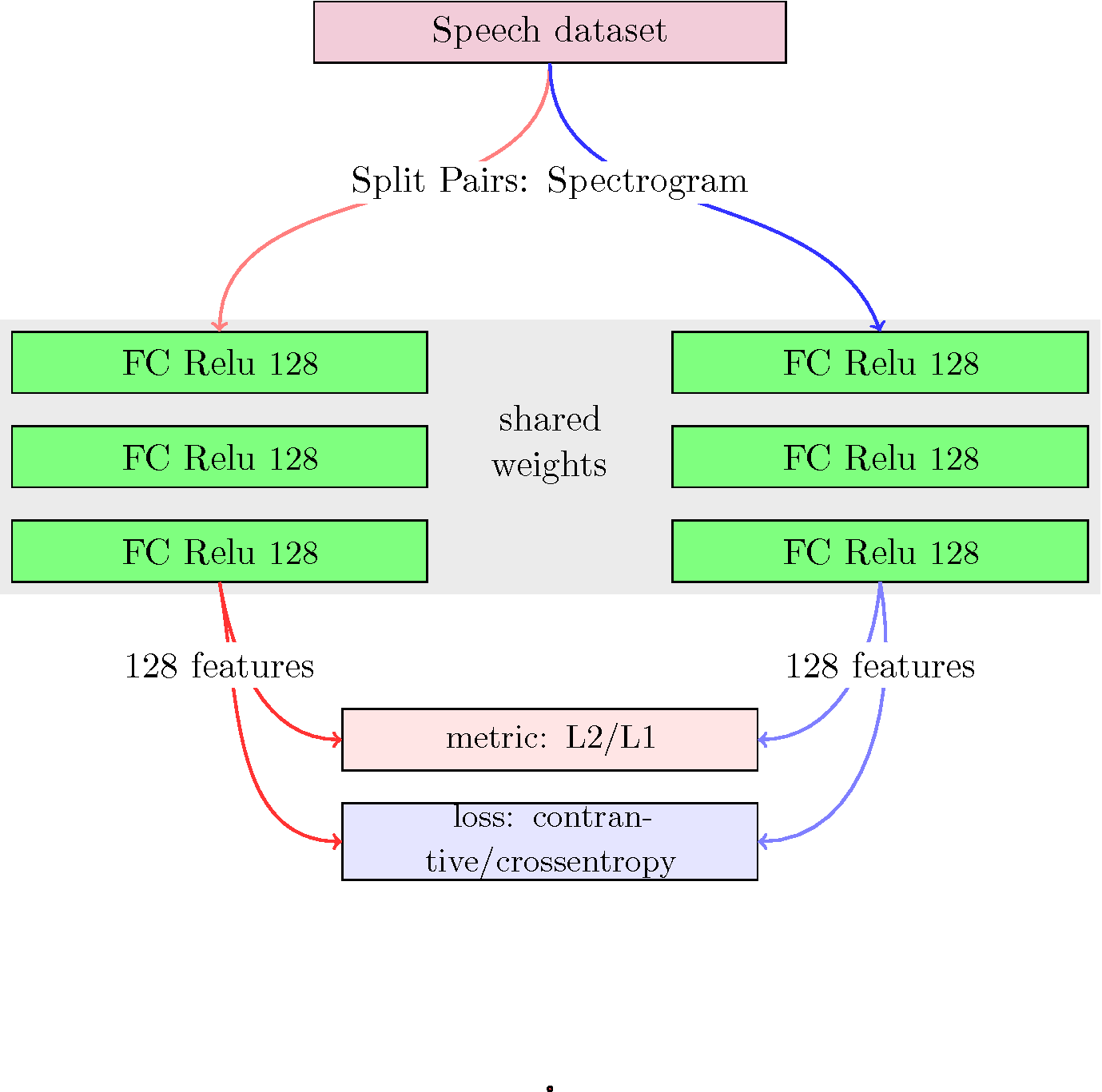
The average accuracy on the test set after 100 epochs is 54.79 %, and 56.87 % on the training set. For this configuration we use the contrastive loss with L2 metric.
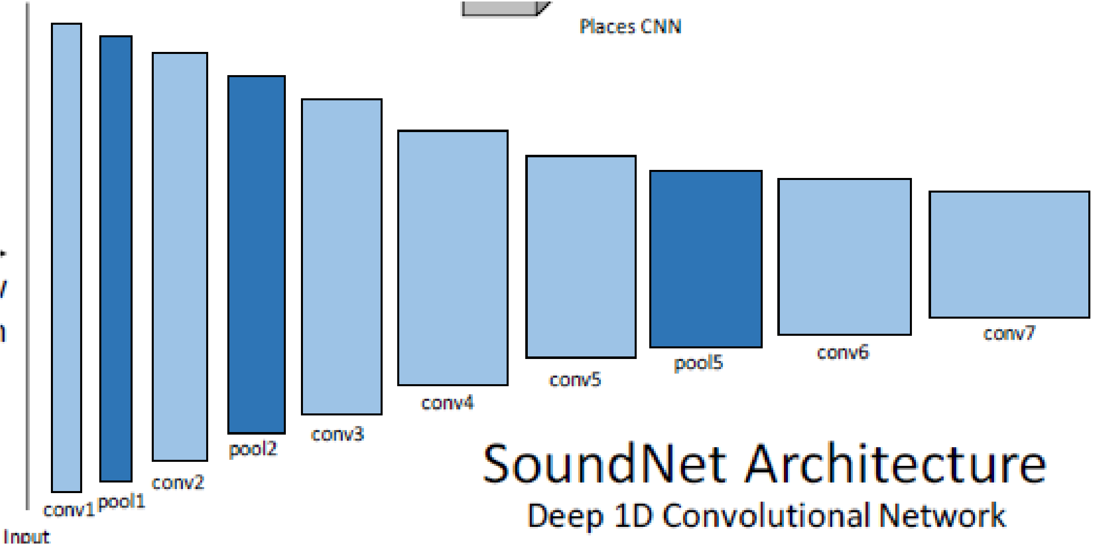
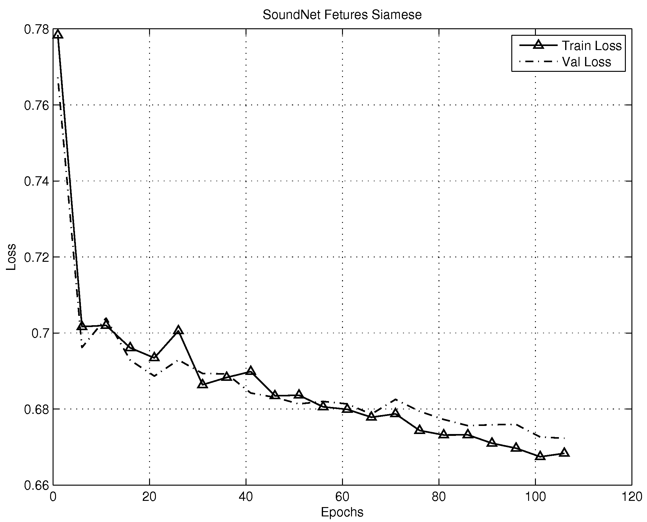
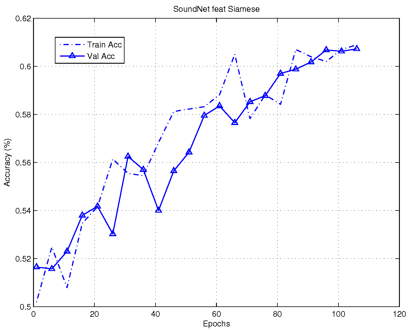
To understand if a more deeper structure will be beneficial for the siamese network we combine the feature extracted by the SoundNet @Aytar2016 architecture with a dense siamese structure. In this case the SoundNet is pretrained with a different dataset for a different classification task as in @Aytar2016. We use this offline model to extract the features. Although, the network is not finetuned for our dataset we believe that the deeper structure can extract feature good enough for the verification process. As we can see from the Figure [fig:3] the performance outperform the baseline siamese network. The average accuracy on the test set is 62.87 % and 65.38 % on the training set.
The performance of this
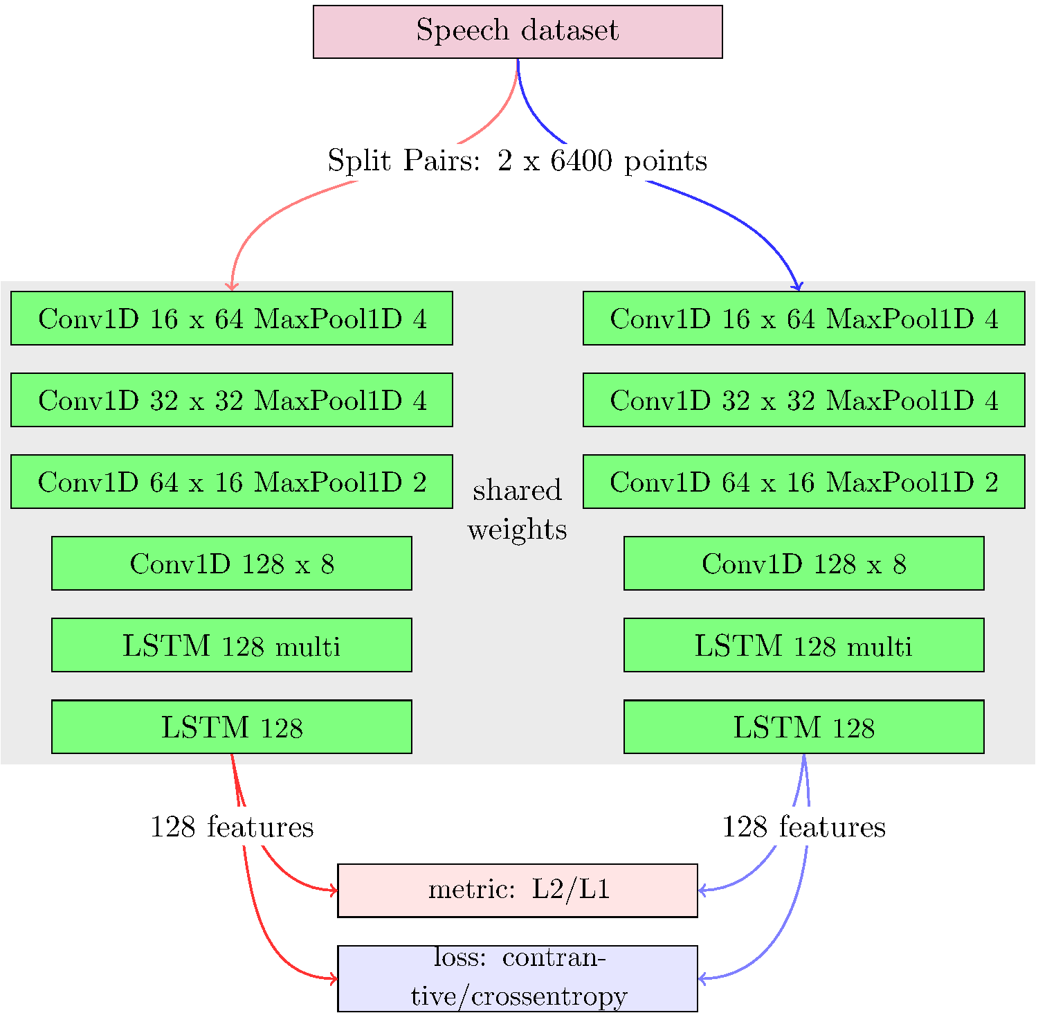
The proposed architecture combine different structure in siamese fashion. We want to take advantage of the Long-Short-Term-Memory unit for its extraordinary performance on temporal data. LSTM is ideal for time series data like sounds, because it can retain the important information of the signal and forget pauses or unimportant data. Unfortunately the raw audio signal can be too heavy to be directly analyzed by the LSTM. Typical audio signals are sampled at 44100 Hz for cd quality, and 16000 Hz for audio. LSTM are trainable with good performance when the sequence is less than 300 sample. Unfortunately 300 samples at 16000 Hz is equivalent to 18 ms, that is quite short for phoneme recognition. To create a low dimensional representation we process the raw signal with one dimensional convolution, and one dimensional MaxPooling. We show the network in Figure [fig:net3], and the footprint on memory on Tables [tab:1],[tab:2]. The convolution block preceding the LSTM will compress the long signal in a more concise and richer feature set. There are two LSTM in cascade working differently. The first one is letting the sequence pass to the second LSTM but working like an accumulator, and memory storage. The second LSTM instead will convert the sequence in a unique vector.
One Leg Siamese configuration
| Layer type | Output shape | # Param | Connected to |
|---|---|---|---|
| Input | (6400,1) | - | - |
| L1 Conv1D 16 x 64 | (6337,16) | 1040 | input |
| L1 MaxPool1D 4 | (1584,16) | 0 | L1 Conv1D |
| L2 Conv1D 32 x 32 | (1553,32) | 16416 | L1 MaxPool1D |
| L2 MaxPool1D 4 | (338,32) | 0 | L2 Conv1D |
| L3 Conv1D 64 x 16 | (373,64) | 32832 | L2 MaxPool1D |
| L3 MaxPool1D 2 | (186,64) | 0 | L3 Conv1D |
| L4 Conv1D 128 x 8 | (179,128) | 65664 | L3 MaxPool1D |
| L5 LSTM 128 x 179 | (179,128) | 131584 | L4 Conv1D |
| L6 Dropout 0.5 | (179,128) | 0 | L5 LSTM |
| L7 LSTM 128 x 1 | (1,128) | 131584 | L6 Dropout |
| L8 FC 128 x 1 | (1, 128) | 16512 | L7 LSTM |
Siamese network configuration.
| Layer type | Output shape | # Param | Connected to |
|---|---|---|---|
| Input 1 | (6400,1) | 0 | - |
| Input 2 | (6400,1) | 0 | - |
| Conv Lstm | (1,128) | 395632 | input 1, input 2 |
| L1 metric | (1,1) | 0 | Conv Lstm 1, Conv Lstm |
| FC | (1,128) | 129 | L1 metric |
| Total # params: | 395761 |
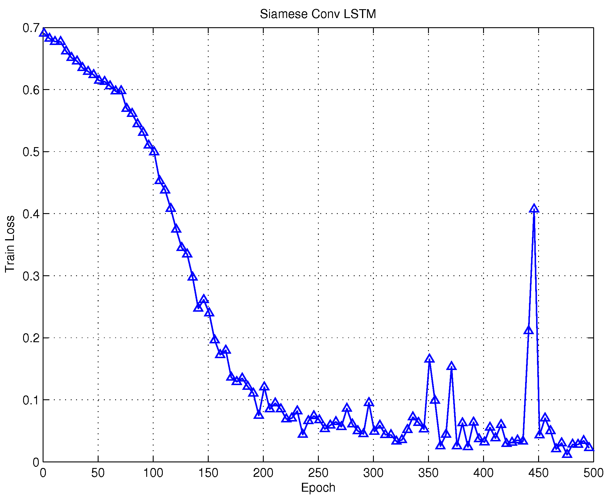
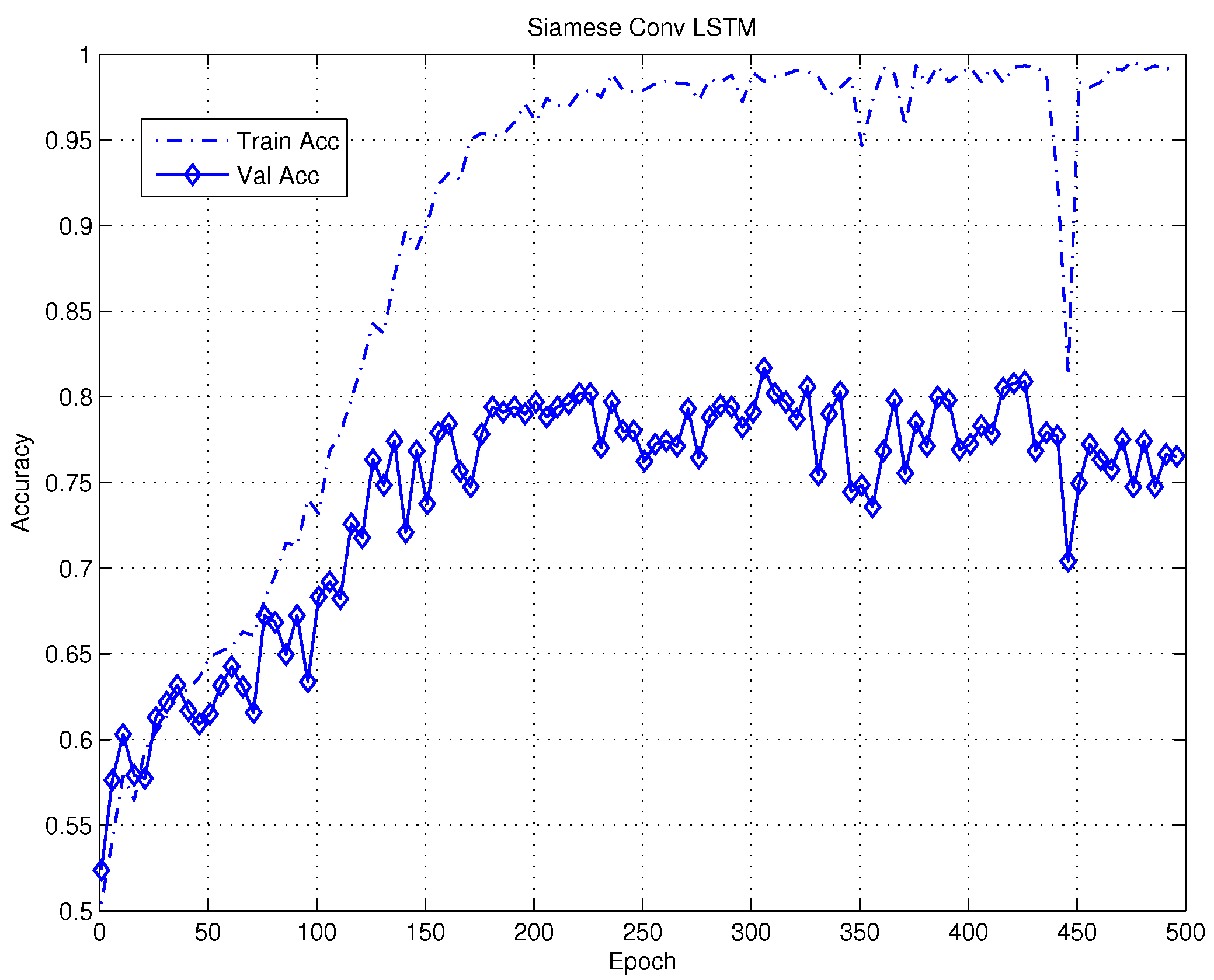
The network has been trained with the raw signal from the speech dataset, as described above. In Figure [fig:5] we show the training loss and accuracy on the train and validation data. We use rmsprop as algorithm for training the network obtaining the accuracy of $~77 \%$ on the validation set, and $98 \%$ on the training set.
We proved a slightly different architecture eliminating the fully connected stage after the second LSTM obtaining the average accuracy of roughly 84 % in the test set.
 Marco Piccirilli